
Universe Scale Serving of Generative Models
And Why You Might Not Want To Use FastAPI For That Purpose

Posted by Javier Mermet
on April 12, 2023 · 10 mins read
New frontiers
If you're a fan of our blog, you know we're constantly pushing ourselves to be at the frontier of AI/ML tech. In our latest technical post, we introduced Stable Diffusion. Not because of all the hype around it, but because our brand-new Research Squad has been doing ✨ magic ✨ with it!
But building on top of state of the art models is not enough by itself if you plan on using it in production. Very much alike other ML projects, for this endeavor to thrive, we had to build the capabilities for serving, monitoring and scaling the infrastructure that will serve as the backbone of the model. This was new ground for us, so we took it one step at a time. We started building from the ground up, learning along the way different alternatives towards getting the most out of available hardware in serving GPU intensive models such as Stable Diffusion.
Goals of our tests
Before doing any benchmarks, we need to know what we'll be optimizing for. In serving a model such as Stable Diffusion, the GPU is most likely to be your hardware bottleneck, whether you are going with cloud providers or on-premise. So, constrained to a given GPU, we want to get the highest throughput possible. That's to say: the most images per second or the most requests per second. These two are similar premises but have a nuanced difference: a request might demand more than one image. So, let's focus on RPS under the assumption that each request requires to generate just one image.
Slow start: FastAPI
FastAPI is a wrapper on top of Starlette, which has gained popularity over the last few years in the Python ecosystem. Many tutorials for Machine Learning practitioners teach you how to serve your models through a RESTful interface using FastAPI, but most lack a complete outlook into the MLOps aspect of it.
FastAPI falls short in many aspects for our purposes:
- Performance
- Ranking: This benchmark is quite popular, and you might notice something not so curious. Python frameworks do not rank well. So, already, the language of choice is not optimal.
- (Micro) Batching: Since FastAPI is not built with the explicit purpose of serving ML models, microbatching is not a built-in feature. You will have to either build it yourself or use a third party package.
- Observability: FastAPI is just a web framework. As such, it doesn't bundle features that enable MLOps/Devops teams to monitor the near real-time status of an app.
- ASGI goes only as far as your GPU/s: The hardware bottleneck in your system will most likely be the GPU, so you want to make the most out of it. There are some optimizations to be made in the API itself, but you'll have to consider how to use the GPU to it's fullest.
Addressing performance
FastAPI optimizations
- Don't use
StreamingResponse. Seriously. Most online tutorials return the generated images usingStreamingResponse, but there are several reasons not to. Using a plainResponse, we saw improvements ranging from 5% for the single user scenario and up to 60% on median latency for the multi user scenario. - Use microbatching. We had to implement this ourselves, but the idea is that you can generate several images with different prompts all at once (provided some other parameters are the same) and we make better use of the GPU. Generation is blocking, so we can serve more requests at once.
- We set two parameters here: the maximum time to wait before fetching the next batch and the maximum number of prompts to fetch. 500ms and 8 prompts seemed like sensible defaults to start with.
Uvicorn workers
- Use
uvloop. By addinguvicornas a dependency with thestandardextras, you getuvloop, which increases performance.
PyTorch optimizations
- Enable attention slicing for VRAM savings
- Enable memory efficient attention for performance
- Enable cuDNN auto-tuner
- Disable gradients calculation
- Set PyTorch's
num_threadsto 1
Implementing observability
Out of the box, FastAPI has no observability capabilities. But there are lots of packages that add features and can be seamlessly integrated.
Prometheus
Prometheus is an open-source systems monitoring and alerting toolkit originally built at SoundCloud. Prometheus collects and stores its metrics as time series data, i.e. metrics information is stored with the timestamp at which it was recorded, alongside optional key-value pairs called labels.
It is widely used to collect metrics as time series and query them through PromQL.
We will be using cadvisor to export metrics from our containers into prometheus, dcgm-exporter to export GPU metrics and as we will see later, metrics straight from FastAPI. For each of these, we use the default scrape_interval of 15 seconds.
Grafana
We set up two dashboards, for different purposes: monitoring the GPU and the API container.
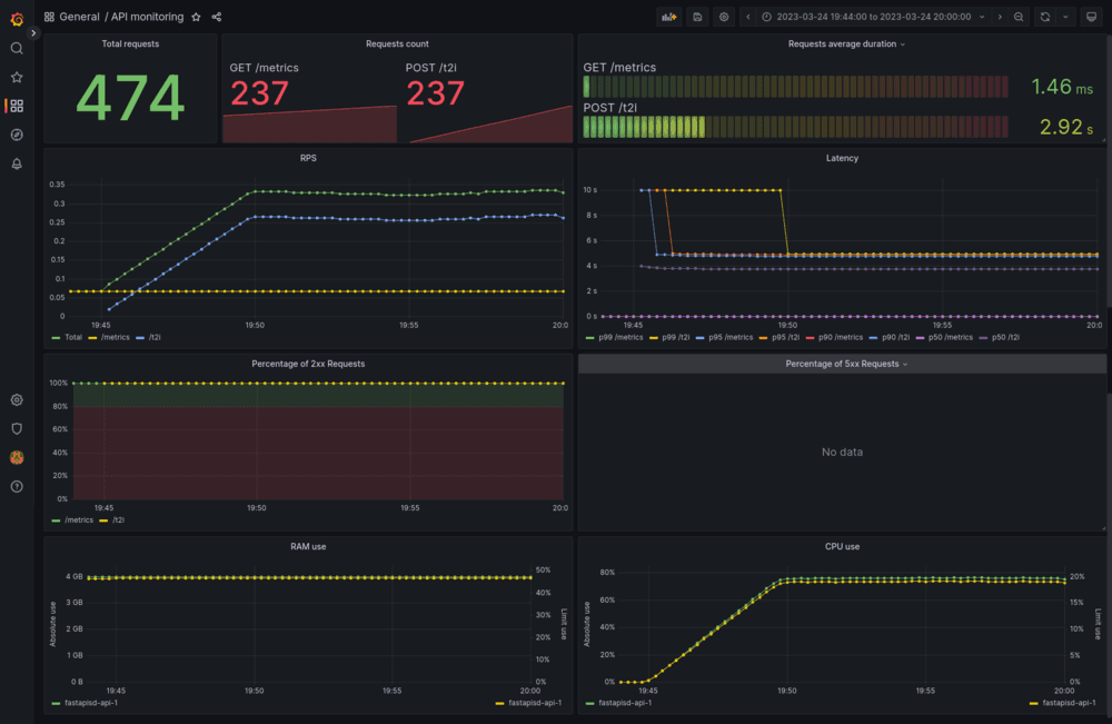

These are a must have for monitoring in a production environment. You need to be able to tell what's wrong with a quick glance.
FastAPI Prometheus instrumentator
We used prometheus-fastapi-instrumentator to add a /metrics endpoint which exports metrics in a prometheus-friendly format.
We had to add latency and requests metrics, but it was a breeze. Read the docs and you will find most use cases explained.
Stress testing
We evaluated several options to stress test the API under different scenarios and workloads. We needed to easily set scenarios to each endpoint so that we could compare later.
- Artillery. Great performance, configurable with code.
- Apache Bench. Easy setup, wrappable in scripts for different scenarios.
- Apache JMeter. A classic choice.
- Locust. For the pythonista. Easy setup. Configurable with code.
Although it's better suited for more complex workflows than ours, we went with locust because of ease of setup, scenario writing, we get performance measures out of the box (on top of prometheus) and we've used it in the past for several projects.
Locust
The setup for each scenario looked similar to this snippet:
import random

from locust import FastHttpUser, task


class T2IHighRes(FastHttpUser):
    @task
    def fetch_image(self):
        self.client.post(
            "/t2i",
            json={
                "seed": random.randint(0, 1_000_000),
                "negative_prompt": "photography",
                "prompt": "digital painting of bronze (metal raven), automaton, all metal, glowing magical eye, intricate details, perched on workshop bench, cinematic lighting, by greg rutkowski, in the style of midjourney, ({steampunk})",
                "width": 512,
                "height": 512,
                "inference_steps": 20,
                "guidance_scale": 8.2,
                # "n": 1,
            },
        )
(Which produces stunning images, by the way)
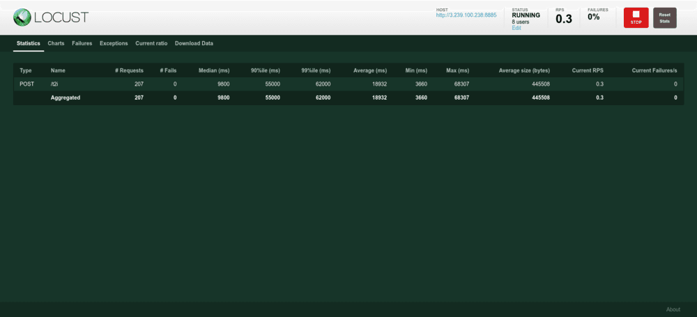
You'll notice that we get many metrics that we already had in grafana. We used both as a double check, but with grafana/prometheus you can get more stylized metrics, such as 5 minutes windows moving averages.
Experiments & Results
We conducted all experiments on g4dn.xlarge spot instances provided by AWS, using the Amazon Linux 2 AMI with Nvidia drivers. Initially, we tried deploying on vast.ai, but we found that it was not possible to run Docker containers due to environment limitations (docker in docker is not available). So, it was not suited for our choice of deployment.
g4dn.xlarge instances have 16GB of RAM, 4 vCPUs and a Nvidia Tesla T4 GPU.
There are five endpoints to generate images, four of them are based on combining these traits:
- Sync vs Async: When using FastAPI, you usually define endpoints as
asyncfunctions, but many times, the underlying service is notasync(for instance,sqlalchemyquerying). We tested whether defining the endpoint+service asasyncfunctions made any difference. - Stream response vs Response: As stated before, we felt this was necessary to test due to how ubiquitous using a
StreamingResponseto return images is on online tutorials and reference implementations. We implemented the same endpoint twice, once using a plainResponseobject and another usingStreamingResponse
And the fifth one is the microbatching endpoint, which uses a custom priority queue to serve a configurable amount of responses at the same time. As said before, the batch timeout are set to 500ms by default and the max batchsize is set to 8. This means that every 500ms, if no group of requests has accumulated 8 requests, we fetch the group with the oldest request and serve those first. Requests are grouped by width, height, inference_steps, and guidance_scale.
For all scenarios we got 0 failures, thus they are not reported. Metrics reported here come from Locust, but where revised against the aforementioned dashboards.
Scenario 1
With only 1 user, for 15 minutes.
{: .table .table-striped .margin-left:auto .margin-right:auto .table-hover .text-nowrap}
| Implementation | Requests | Avg (ms) | RPS | p50 (ms) | p90 (ms) | p95 (ms) | p99 (ms) |
|---|---|---|---|---|---|---|---|
| Streaming (Async) | 218 | 4112 | 0.2 | 4100 | 4200 | 4200 | 4200 |
| Response (Async) | 230 | 3912 | 0.3 | 3900 | 4000 | 4000 | 4000 |
| Streaming (Sync) | 226 | 3978 | 0.3 | 4000 | 4000 | 4000 | 4200 |
| Response (Sync) | 236 | 3811 | 0.3 | 3800 | 4000 | 4000 | 4000 |
| Batched (Async) | 368 | 2439 | 0.4 | 2400 | 2400 | 2400 | 2400 |
Even without the bolding, you can see there's a clear winner. The microbatching implementation, albeit a very simple one, greatly improves both latency and throughput. And this is even without trying to optimize the microbatching configuration from the "sensible defaults" mentioned before.
Another clear insight for this use case is that using StreamingResponse harms performance. Async/Sync implementation of endpoints and generation functions make no difference.
But how does each implementation fare respecting to GPU usage? Let's check some metrics obtained from the Grafana dashboard.
{: .table .table-striped .margin-left:auto .margin-right:auto .table-hover .text-nowrap}
| Implementation | GPU Avg VRAM Use | GPU Avg Utilization |
|---|---|---|
| Streaming (Async) | 80.6% | 68.8% |
| Response (Async) | 60.8% | 59.3% |
| Streaming (Sync) | 59.7% | 71.0% |
| Response (Sync) | 58.5% | 63.1% |
| Batched (Async) | 75.1% | 42.8% |
While one could make a point that using the most GPU is better, measuring that becomes tricky. For instance, the Sync Streaming endpoint uses more than the batched one, but results in lower throughput and higher latency.
Scenario 2
One could argue the above scenario is not quite representative of the workload a production-ready API might encounter. So, we built another scenario. 8 users, with a spawning rate of 0.02 users/second (a new user arrives every 50 seconds), for 15 minutes.
{: .table .table-striped .margin-left:auto .margin-right:auto .table-hover .text-nowrap}
| Implementation | Requests | Avg (ms) | RPS | p50 (ms) | p90 (ms) | p95 (ms) | p99 (ms) |
|---|---|---|---|---|---|---|---|
| Streaming (Async) | 261 | 21951 | 0.3 | 26000 | 28000 | 34000 | 46000 |
| Response (Async) | 269 | 20875 | 0.3 | 9900 | 53000 | 56000 | 69000 |
| Streaming (Sync) | 264 | 21618 | 0.3 | 26000 | 32000 | 34000 | 46000 |
| Response (Sync) | 270 | 20729 | 0.3 | 9800 | 56000 | 59000 | 65000 |
| Batched (Async) | 975 | 5923 | 1.1 | 6400 | 6500 | 6500 | 12000 |
This scenario gives further evidence of our prior conclusions.
{: .table .table-striped .margin-left:auto .margin-right:auto .table-hover .text-nowrap}
| Implementation | GPU Avg VRAM Use | GPU Avg Utilization |
|---|---|---|
| Streaming (Async) | 87.7% | 92.1% |
| Response (Async) | 84.2% | 91.9% |
| Streaming (Sync) | 90.6% | 93.6% |
| Response (Sync) | 60.2% | 87.7% |
| Batched (Async) | 71.3% | 80.3% |
The batched implementation has no bottleneck in the GPU, which is a good thing: we should be able to keep scaling to more users.
Transformers optimizations.
In these tests, we tested the impact that had enabling and disabling Memory Efficient Attention (MEA) and Attention Slicing (AS).
We used the same ramp up as in scenario 2: 8 users, with a spawning rate of 0.02 users/second, for 15 minutes.
{: .table .table-striped .margin-left:auto .margin-right:auto .table-hover .text-nowrap}
| MEA | AS | Requests | Avg (ms) | RPS | p50 (ms) | p90 (ms) | p95 (ms) | p99 (ms) |
|---|---|---|---|---|---|---|---|---|
| ✅ | ✅ | 975 | 5923 | 1.1 | 6400 | 6500 | 6500 | 12000 |
| ❌ | ❌ | 932 | 6200 | 1 | 6900 | 7000 | 7000 | 11000 |
| ❌ | ✅ | 957 | 6040 | 1.1 | 6500 | 6700 | 6800 | 13000 |
| ✅ | ❌ | 1131 | 5102 | 1.3 | 5300 | 5800 | 5800 | 8800 |
And as for GPU impact:
{: .table .table-striped .margin-left:auto .margin-right:auto .table-hover .text-nowrap}
| MEA | AS | GPU Avg. VRAM | GPU Avg. Utilization |
|---|---|---|---|
| ✅ | ✅ | 71.3% | 80.3% |
| ❌ | ❌ | 72.7% | 87.4% |
| ❌ | ✅ | 63.9% | 82.5% |
| ✅ | ❌ | 49.9% | 83.8% |
In our tests, enabling memory efficient attention and disabling attention slicing had the best results. Which is why we used that config in the next test.
Additionally, we tried using Channels Last memory format for NCHW tensors, and improved even further these results:
{: .table .table-striped .margin-left:auto .margin-right:auto .table-hover .text-nowrap}
| Requests | Avg (ms) | RPS | p50 (ms) | p90 (ms) | p95 (ms) | p99 (ms) |
|---|---|---|---|---|---|---|
| 1316 | 4383 | 1.5 | 4800 | 5100 | 5300 | 5400 |
Batched parameters optimization
By now, we have full evidence that even the most basic of microbatching implementations can greatly improve our target metrics. Can we get better numbers by playing around with some parameters? We tried increasing/decreasing both the batch timeout and batch max size. Same as previous test, we set 8 users to arrive at a rate of 0.02 users/second, and ran the test for 15 minutes.
{: .table .table-striped .margin-left:auto .margin-right:auto .table-hover .text-nowrap}
| Batch Timeout (ms) | Batch Size | Requests | Avg (ms) | RPS | p50 (ms) | p90 (ms) | p95 (ms) | p99 (ms) |
|---|---|---|---|---|---|---|---|---|
| 500 | 8 | 1131 | 5102 | 1.3 | 5300 | 5800 | 5800 | 8800 |
| 250 | 8 | 1121 | 5145 | 1.2 | 5400 | 6000 | 6000 | 9700 |
| 1000 | 8 | 1030 | 5599 | 1.1 | 5900 | 6000 | 6000 | 12000 |
| 500 | 4 | 1083 | 5331 | 1.2 | 5900 | 5900 | 5900 | 8200 |
| 500 | 16 | 1051 | 5506 | 1.2 | 6000 | 6100 | 6100 | 12000 |
Our takeaway is that those initial "sensible defaults" were... sensible enough. However, were we to take these results at face value, we'd really be overfitting to our test scenario. While changing the batch size can make the median latency 5-10% worse, that might change if we change the number of users.
Conclusions and next steps
While the initial results are exciting, they came at a cost. Mostly in engineering time and implementation of basic features for Deep Learning models serving.
We will be taking Triton for a test ride next, and we have high hopes for it. There are several other alternatives to consider, as this is a growing space. After everything you've read in this article, we have a strong baseline to compare against and a clearly defined methodology and performance indicators that will guide us.